Polynomials
Polynomials
In the module Parametric form we, in a more or less intuitive way, set up the following expression for a line in the plane.
      x(t)=(x2-x1)·t+x1
      y(t)=(y2-y1)·t+y1
We want to generalize this and extend the reasoning to other curves than lines. We stay in the plane.
Linear polynomial
The deduction of the expression above can be generalized like this:
A line is described by:
Q(t)=| x(t),y(t) | = | axt+bx,ayt+by |
We require that the line segment should have endpoints in P1(x1,y1) and P2(x2,y2). This is the constraints for the curve.
This enables us to write:
|
x(0)=bx=x1 |
y(0)=by=y1 |
We have 4 unknown coefficients that we have to find. We solve the two equation pairs and get:
bx=x1
by=y1
ax=x2-x1
ay=y2-y1
The parametric equations for the curve become:
Q(t)=| (x2-x1)t+x1,(y2-y1)t+y1 |
as we set it up intuitively in module: Parametric form.
Quadratic by example
But we aren't satisfied with only lines and circles. We must be able to handle curves of more or less complex nature. When we deal with this, two complications arise:
- We cannot be satisfied with linear expressions for t. We will stick to polynomials as a tool. We know that a 2-degree expression results in a simple curvature, since the derivative is linear. A 3-degree expression can result in two curvatures.
- We have to specify the curve. It is not enough to state the endpoints, as we do for lines.
To solve the last issue we will use the derivative. We study a 2-degree polynomial.
Q(t)=| x(t),y(t) | = | axt2+bxt+cx,ayt2+byt+cy |
Derived with regard to t:
Q'(t)=| x'(t),y'(t) | = | 2axt+bx, 2ayt+by|
We specify the following requirements for the curve:
- It should run through P1(0,0)(origin)
- It should run through P2(6,0)
- The derivative, the vector tangent, in P1 should be R1(0,6)
This results in two equation sets, each with three equations:
|
x(0)=cx=0 |
y(0)=cy=0 |
We notice that we have 6 unknown coefficients that have to be found. We solve the equations and get:
ax=6
bx=0
cx=0
ay=-6
by=6
cy=0
The parametric equation for the curve becomes
Q(t)=|6t2,-6t2+6t|
and the derivative
Q'(t)=|12t,-12t+6|
We insert some t-values:
| Q(0) | (0,0) as we wanted |
| Q(0.25) | (0.375,1.125) |
| Q(0.5) | (1.5,1.5) |
| Q(0.75) | (3.375,1.125) |
| Q(1) | (6,0) as we wanted |

We notice that when we have a 2.order expression we will get a simple curvature since the derivative is linear. If we want more advanced curve shapes, we need a higher degree polynomial.
Cubic by example
We are still in the plane and we want to make a cubic form on the parametric curve.
Q(t)=| x(t)=axt3+bxt2+cxt+dx,y(t)=ayt3+byt2+cyt+dy|
When we have a cubic expression we can get a more complicated curve since the derivative is of 2-degree. We also notice that we have 8 unknown coefficients that have to be found.
The following is specified for the curve:
- It should run through origin, P1(0,0)
- It should run through P4(6,0)
- The derivative, the tangent vector, in P1 should be R1(0,6)
- The derivative, the tangent vector, in P4 should be R4(0,6)
(We'll use P1 and P4 for endpoints to work in a terminology that makes it easier to compare it with other geometrical specifications later.)
This results in two equation sets, each with four equations:
|
x(0)=dx=0 |
y(0)=dy=0 |
We solve and get
ax=-12
bx=18
cx=0
dx=0
ay=12
by=-18
cy=6
dy=0
The parametric equations for the curve are
x(t)=-12t3+18t2
y(t)=12t3-18t2+6t
and
x'(t)=-36t2+36t
y'(t)=36t2-36t+6
We'll insert some t-values:
| Q(0) | (0,0) as we wanted |
| Q(0.25) | (0.937,0.563) |
| Q(0.5) | (3.0,0.0) |
| Q(0.75) | (5.1,-0.563) |
| Q(1) | (6,0) as we wanted |
The Hermit curve
The conditions we set in example 2, specifying the endpoints and the derivative in both endpoints, gives us a named type of curves: Hermit curve. We generalize our reasoning to 3D and write:
Q(t)=| x(t),y(t),z(t) | =| axt3+bxt2+cxt+dx , ayt3+byt2+cyt+dy, azt3+bzt2+czt+dz |
and
Q'(t)=| x'(t),y'(t),z'(t) | =| 3axt2+2bxt+cx, 3ayt2+2byt+cy, 3azt2+2bzt+cz |
We concentrate about x(t) and set up the current general equation set:
      x(0)= d = P1
      x(1)= a+b+c+d = P4
      x'(0)= c = R1
      x'(1)= 3a + 2b + c = R4
where P1 stands for P1's x-component and so on.
We see that d=P1 and c=R1 . We substitute these values in the other two equations and get the following to solve:
      a+b+R1+P1=P4
      3a+2b+R1=R4
And the solution is:
      a=2P1-2P4+R1+R4
      b=-3P1+3P4-2R1-R4
      c=R1
      d=P1
This gives us:
x(t) =t3(2P1-2P4+R1+R4)+t2(-3P1+3P4-2R1-R4)+t(R1)+P1
=P1(2t3-3t2+1) + P4(-2t3+3t2)
+ R1(t3-2t2+t) + R4(t3-t2)
We get the same expressions for y(t) and z(t). We notice that x(0)=P1 and x(1)=P4.
When they are written in this form we notice that the four geometric conditions, P1, P4, R1, R4 are weighed with cubical t-polynomials.
The blending functions, t-polynomials, are like this in the area t [0..1]:

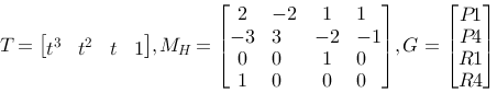
We want to use this way of thinking and want to separate the geometric conditions and the four weight functions or blending functions. We will try with a matrix shape where we separate the geometric conditions from the weights.
Q(t)=| x(t) , y(t) , z(t) |= T·MH·G
Where G expresses the geometric guidelines and M express the weight functions.