
The Bezier curve
In the module Polynoms we have solved a general problem which is to calculate a polynomial of third degree based on geometrical guidelines. The Hermit curve is the solution, based on us knowing the curve's endpoints and the derived in those endpoints. We have also found a general form to express a curve like this: T·MH·G.
A curve of third degree
We'll use a situation quite similar to the one we had when we developed the Hermit curve
in the module Polynoms.
We want to find the coefficients in an expression in the third degree:
B(t)=at3+bt2+ct+d
We want geometrical guidelines that state that the curve should start and stop in two decided points, P0 and P3. Consequently: B(0)=P1 and B(1)=P3. We want a polynomial of third degree and need two more guidelines. We use two points that indirect state the derivative in the endpoints:

|
We decide that B'(0)=3(P1-P0) B'(1)=3(P3-P2) |
The derivative is: B'(t)=3at2+2bt+c
We have to find a,b,c and d in this equation:
      B(0)=d=P0
      B(1)=a+b+c+d=P3
      B'(0)=c=3(P1-P0)
      B'(1)=3a+2b+c=3(P3-P2)
We solve and find:
      a=-P0+3P1-3P2+P3
      b=3P0-6P1+3P2
      c=3P1-3P0
      d=P0
and we set up the expression for B(t):
B(t)=-P0t3+3P1t3-3P2t3+P3t3+3P0t2-6P1t2+3P2t2+3P1t-3P0t+P0
We rearrange and get:
B(t)=P0(-t3+3t2-3t+1)+
P1(3t3-6t2+3t)+
P2(-3t3+3t2)+
P3(t3)
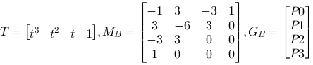
This has given us a form that resembles the one we had for the Hermit curve and we can set up the expression in a matrix form:
B(t) =T·MB·GB
where
The blending functions are described like this:
|
P0: -t3+3t2-3t+1 |

|
You can experiment with the Bezier curve below
Let us ascertain that we can rewrite:
B(t)=P0(-t3+3t2-3t+1)+
P1(3t3-6t2+3t)+
P2(-3t3+3t2)+
P3(t3)
to

which is the shape the Bezier curve usually is shown. More about this below.
de Casteljau
We can find the Bezier curve in another way as well, with the de Casteljau algorithm.
The starting point is the parametrical shape on a line that is in way so that P(0)=P0 and P(1)=P1: P(t)=(1-t)P0+tP1. A reasoning based on de Casteljau's algorithm leads to this being perceived as special case of a Bezier curve, a linear Bezier curve.
The algorithm can be described after the following scheme, where we imagine that t runs from 0 to 1:

|
P(t)=(1-t)P0+tP1 |

|
P(t)=(1-t)A(t)+tB(t) and: A(t)=(1-t)P0+tP1 B(t)=(1-t)P1+tP2 We fill in and get: P(t)=(1-t)2P0+2t(1-t)P1+t2P2 |

|
P(t)=(1-t)D(t)+tE(t) and:
D(t)=(1-t)A(t)+tB(t) and:
A(t)=(1-t)P0+tP1 We fill in two rounds and get: P(t)=(1-t)3P0+3t(1-t)2P1+3t2(1-t)P2+t3P3 |
The last expression is the same as the one we reached above, when we used a general polynomial of third degree and constraints for the endpoints and the derivative in the endpoints as a starting point.
It is easy to convince oneself that we can repeat the de Casteljau algorithm with further control points, P4, P5 etc.
You can animate the de Casteljau algorithm with 4 control points in the applet below. Move the points and start the animation.
(A stunt applet by Håvard Rast Blok, noon - 15.2.2001 )
Summed up
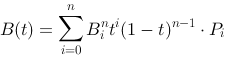
The expression for the Bezier function is in general:
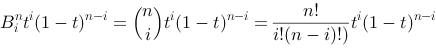
where n states the number of control points.
The description of the curve becomes:
Coefficients, are the same as the ones in Pascal's triangle:
| 1 | ||||||||
| 1 | 1 | |||||||
| 1 | 2 | 1 | ||||||
| 1 | 3 | 3 | 1 | |||||
| 1 | 4 | 6 | 4 | 1 |
We have used n=4, and used the coefficients 1, 3, 3, 1.
Curve segments
The general shape of the Bezier curve gives us the possibility to specify more control points. We can for example let n=5 and get:

We will not develop this reasoning to handle longer curves. We will in stead regard a curve as put together by several curve segments.
We want to look at how we can join curves and gain different degrees of smoothness. We will concentrate on what conditions that has to be fulfilled if two segments are going to hang together in a "smooth" way. We'll look at four degrees of geometric continuity. We'll regard Bezier curves and represent them as they are represented in drawing programs. The lines between the control points is represented as "handles" that we can use to change the shape of the curve.

|
No continuity. The two curve segments don't have a common point. |

|
The two curve segments have a common point. The curves are connected, but with an obvious break in direction. The derivatives (for right and left segment) are different both in direction and size in this point. |

|
The two curve segments have a common point, and the joint is quite smooth. The derivatives in this point have the same direction, but not the same size. |

|
The two curve segments have a common point, and the joint is smooth. The derivatives in this point have the same direction and size. |
Calculation
Even though OpenGL have mechanisms to draw Bezier surfaces, it is often convenient to draw Bezier curves "by hand". Maybe we want to use the curve in an ordinary window, without OpenGL. Often connected with an interactive manipulation of the control points. Then it is useful to find an effective way to calculate an adequate number of points on the curve to create a shape that is smooth enough to watch.
If we decide that the resolution is permanent, lets say that we want to calculate the curve for m t-values inclusive 0 and 1. We see from the expression for the curve that we can calculate and tabulate m values of (1-t)3, (1-t)2, (1-t), t3, t2, t. In total a 6 x m table. If the control points move, we can calculate the new curve with help from the table.
In addition we only have to calculate values in the t-area where the new curve is significantly, visibly, different from the old one. Indeed we see from the Bezier curve's weight functions that all control points affects a whole curve segment, but the difference can be smaller than what's visible on the screen. This requires that we keep the old curve to be able to compare them.
Surfaces
We can generalize Bezier curves to Bezier surfaces. In this case we imagine control points in a net, and we can calculate curves along both directions in the net and interpolate. OpenGL handles this.
In OpenGL
Bezier curves is handled directly by OpenGL
    // 4 control points in space
    GLfloat ctrlpoints[4][3] = {
        {-4.0,-4.0,0.0},
        {-2.0,4.0,0.0},
        {2.0,-4.0,0.0},
        {4.0,4.0,0.0}    };
    // we want to draw with t from 0.0 to 1.0
    // and we give the dimensions of the data
    glMap1f(GL_MAP1_VERTEX_3,0.0,1.0,3,4,& ctrlpoints[0][0]);
    glEnable(GL_MAP1_VERTEX_3);
    // draw a curve with 30 steps from t=0.0 to t=1.0
    glBegin(GL_LINE_STRIP);
    for (int i=0;i<=30;i++)
       glEvalCoord1f((GLfloat) i/30.0);
    glEnd();
Example of a surface definition and drawing.
   // define ctrlpoints for trampoline
  GLfloat ctrlpoints[4][4][3] = // [v][u][xyz]
  {
   { {-1.5f,-1.5f,0.0f}, {-0.5f,-1.5f,0.0f},
     {0.5f,-1.5f,0.0f}, { 1.5f,-1.5f,0.0f}
   },
   { {-1.5f,-0.5f,0.0f}, {-0.5f,-0.5f,0.0f},
     {0.5f,-0.5f,0.0f}, {1.5f,-0.5f,0.0f}
   },
   {{-1.5f,0.5f,0.0f}, {-0.5f,0.5f,0.0f},
    {0.5f,0.5f,0.0f}, {1.5f,0.5f,0.0f}
   },
   { {-1.5f,1.5f,0.0f}, {-0.5f,1.5f,0.0f},
     {0.5f,1.5f,0.0f}, {1.5f,1.5f,0.0f}
   }
  };
  ...
  //  drawing
    glMap2f(GL_MAP2_VERTEX_3,0.0f,1.0f,3,4,0.0f,1.0f,12,4,
            & ctrlpoints[0][0][0]);
    glEnable(GL_MAP2_VERTEX_3);
    glMapGrid2f(20,0.0f,1.0f,20,0.0f, 1.0f);
    glEvalMesh2(GL_FILL, 0, 20, 0, 20);
