
NURBs
Uniform Non Rational B_splines
We start out with a situation that may be characterized as Uniform Non Rational B-splines.

We have m+1=8 control points, and m-2=5 curve segments. The curve may be described by a parameter running from t3 to t8. A curve segment is limited by one t-step. The curve Qi is described by t running from ti to ti+1.
The segments are coupled according to this scheme:
- Q3 depends on P0 ,P1 ,P2 ,P3
- Q4 depends on P1 ,P2 ,P3 ,P4
- Q5 depends on P2 ,P3 ,P4 ,P5
- ...
- Qi depends on Pi-3 ,Pi-2 ,Pi-1 ,Pi
Each curve is described by 4 control points. This means that we have local control in the sense that no other points than those 4 influence the curves shape. In the same manner we see that each control point is involved i 4 curve segments.
we note that this is interesting compared to what we can achieve with Bezier curves. If we wanted a Bezier curve with the same amount of control points we would have to increase the level of the curve to m-1 and we would have a situation where all control points would influence the curve as such. If we make a curve by connecting cubical Bezier curves, we would have local control, but we would not control the continuity across segments when we change single control points.
we will look a little closer at the segments. We know from the modules Bezier and Polynoms the general form of a curve or curve segment:
Q(t)=T·M·G,
where T is a row vector describing the level of the curve, M is a 4x4 matrix which is special for the curve form and G is column vector describing the geometrical restrictions.
For curve segment i we can write:
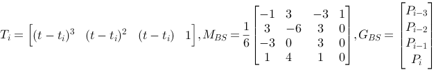
There are two things to note here.
Firstly we have not made any argument for the matrix itself MBS.
Secondly we have a T vector which is a little more complicated than those we know from Hermit and Bezier, since we have (t-ti) in stead of t. we can, without loosing generality, replace (t-ti) with t, and thus achieve the same T·M for all curve segments. we know that this product will give us 4 weight functions which in turn tells us how strong influence each of the 4 control points has on the curve when t runs from 0 to 1. For B-Splines the weight functions will be:

|
Vi-3 = 1/6(-t3+3t2-3t+1)
Vi-2 = 1/6(3t3-6t2+4)
Vi-1 = 1/6(-3t3+3t2+3t+1)
Vi = 1/6(t3)
|
We use them like this:
 Qi(t)=
       Vi-3·Pi-3 +
       Vi-2·Pi-2 +
       Vi-1·Pi-1 +
       Vi·Pi
This far we have established and described a complete curve form which is uniform in the sense that all curve segments are described in the same way. The t - values are regular in the sense that they "moves us the same amount forward": ti+1 - ti = 1
Non Uniform Rational B-splines
We will now turn our attention to curves that are rational (as above), and Non Uniform.
To say that a curve is "Rational" means that it maybe described in homogenous coordinate system and this has as a consequence that they may be subject to the usual transformations without loosing their form. We will not follow up on this here.
When a curve is "Non Uniform" it means that the single segments of the curve not has the same description and it means that we can manipulate the curve, and especially the continuity between segments by manipulating the t-values. This is what makes NURB's a handy modeling tool. The t-points, or the transition from one segment to the next are called knots. As a special case we can see from the description above that if concatenate two t- values, we eliminate a curve segment. This means that to two neighboring segments on each side will be connected, but the continuity will be changed, and will not be as smooth as in a uniform curve. If we concatenate 4 knots (eliminate 4 curve segments) we will have a discontinuity in the curve. The neighbors on each side will not have a common control point.
The 4 commented illustrations below describes some of the possibilities. (Note that the illustrations are "handmade" and may be inaccurate, the important thing is to emphasis the principles)


In openGL
Curve
   // make a nurb object
   theNurb=gluNewNurbsRenderer();

   expectedError=GLU_INVALID_ENUM;

   // draw nurb,using the nurbobject:theNurb
   gluNurbsProperty(theNurb,GLU_SAMPLING_TOLERANCE,25.0);
   gluNurbsProperty(theNurb,GLU_DISPLAY_MODE,GLU_FILL);
   // defining a callback for errorreport
   gluNurbsCallback(theNurb,GLU_ERROR,
                    (GLvoid(__stdcall *)())errorInNurb);


   glLineWidth(4.0);
   glDisable(GL_LIGHTING);
   glColor3f(0.0,0.0,1.0);
   // displaying
   gluBeginCurve(theNurb);
   gluNurbsCurve(
      theNurb,
      uk_count,      // knot count along u
      u_knots,       // .. and the knots
      3,             // from one u to the next
      & ctpnts[0][0], // the pointarray
      4,             // order of polynomial, cubic+1
      GL_MAP1_VERTEX_3
      );
   gluEndCurve(theNurb);

   gluDeleteNurbsRenderer(theNurb);
Surface
   // make a nurb object
   theNurb=gluNewNurbsRenderer();

   expectedError=GLU_INVALID_ENUM;


   // draw nurb,using the nurbobject:theNurb
   gluNurbsProperty(theNurb,GLU_SAMPLING_TOLERANCE,25.0);
   gluNurbsProperty(theNurb,GLU_DISPLAY_MODE,GL_FILL);
   // defining a callback for errorreport
   gluNurbsCallback(theNurb,GLU_ERROR,
                    (GLvoid(__stdcall *)())errorInNurb);


   // displaying
   gluBeginSurface(theNurb);
   gluNurbsSurface(
      theNurb,
      uk_count,      // knot count along u
      u_knots,    // .. and the knots
      vk_count,      // knot count along v
      v_knots,    // .. and the knots
      VMAX*3,        // from one u to the next
      3,          // from one v to the next
      & ctpnts[0][0][0],
      4,          // order of polynomial, cubic+1
      4,          // order of polynomial, cubic+1
      GL_MAP2_VERTEX_3
      );

   gluEndSurface(theNurb);

   gluDeleteNurbsRenderer(theNurb);
Trimming
OpenGL gives us the possibility to "trim" a NURB surface. That means that we sets up borders for which part of the surface we want to render. We do this by specifying closed polygons by 2D-points within the parameter space. The logic is that the parts of the surface to the left of the polygon will be included, while the parts to the right will be excluded. This it is important that we give the points in the trimming polygon in correct order: we include by giving the points counterclockwise, and remove by giving the points clockwise.
Note that the coordinates of the trimming polygon are given within the curves parameter space, that is within the range of the t-values we use. The actual spatial coordinates are irrelevant in this operation.
   // make a nurb object
   theNurb=gluNewNurbsRenderer();

   expectedError=GLU_INVALID_ENUM;


   // draw nurb,using the nurbobject:theNurb
   gluNurbsProperty(theNurb,GLU_SAMPLING_TOLERANCE,25.0);
   gluNurbsProperty(theNurb,GLU_DISPLAY_MODE,GL_FILL);
   // defining a callback for errorreport
   gluNurbsCallback(theNurb,GLU_ERROR,
                    (GLvoid(__stdcall *)())errorInNurb);


   // displaying
   gluBeginSurface(theNurb);
   gluNurbsSurface(
      theNurb,
      uk_count,      // knot count along u
      u_knots,    // .. and the knots
      vk_count,      // knot count along v
      v_knots,    // .. and the knots
      VMAX*3,        // from one u to the next
      3,          // from one v to the next
      & ctpnts[0][0][0],
      4,          // order of polynomial, cubic+1
      4,          // order of polynomial, cubic+1
      GL_MAP2_VERTEX_3
      );

      // Trimming

      // what we want
      gluBeginTrim(theNurb);
      gluPwlCurve(theNurb,5,& trim_outside[0][0],2,GLU_MAP1_TRIM_2);
      gluEndTrim(theNurb);


      // what we dont want
      gluBeginTrim(theNurb);
      gluPwlCurve(theNurb,5,& trim_inside[0][0],2,GLU_MAP1_TRIM_2);
      gluEndTrim(theNurb);


   gluEndSurface(theNurb);

   gluDeleteNurbsRenderer(theNurb);
