Frames

Problem

Suppose we have a parametric curve C(t). We want to draw a small figure repeatedly with even t-steps along this curve. We can realize this quite easily with code like this:

 while( t < t_max)
 {
   glPushMatrix();
   glTranslate(Cx(t),Cy(t),Cz(t));
   < Draw figure >
   glPopMatrix();
   t+=t_step;
 }
 	

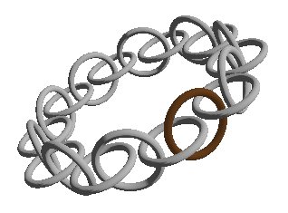
This works fine as long as we don't have any demands about how the figure is oriented in proportion to the curve, or as long the figure don't have any orientation. For example a pearl necklace of completely round pearls could easily be drawn this way.

If the figure has an orientation we have to modify the algorithm:

 while( t < t_max)
 {
   tglPushMatrix();
   glTranslate(Cx(t),Cy(t),Cz(t));
   < rotate the figure to its place >
   < draw figure >
   glPopMatrix();
   t+=t_step;
 }
	

The problem here is that the line that rotates the figure to its place can be quite hard to replace with code. This is the problem we shall find a general solution for.

What we want is a transformation that transforms us to a coordinate system on the curve; to the place we desire and with the axis directions we want.

The method

The method lets us decide the directions for the axes we want in the new coordinate system, and then it puts these directions, together with information about the new origin, into a matrix. The method is described step by step below:

1. We will start with finding a vector T that describes one of the axes in our desired coordinate system. In most cases it is reasonably that one of the axes lies "along" the curve. In other words, we want to use the curve's derived as an axis: T(t)=C'(t). We'll only write T from now on, and we'll assume that all the vectors are calculated for a certain t-value.

2. Then we want to determine a vector B that is normal to the one we picked in the first step above. We'll have to decide which direction to choose. We can in principle choose any vector V, and find B as the cross product of T and V: B=T X V. The only formal demand we set for V is that it doesn't coincide with ( is co-linear with) T. If this condition is met we know that the cross product above gives us a vector that is a normal to T (and V). The choice of T is decisive for the orientation of the to other axes in the coordinate system. One suggestion is the to use the double derivative of C(t),C''(t), if this exists. We'll study this in the examples below.

3. Now we want to decide upon a third vector, N, this is normal to both T and B. The choice we made in the second section decides the third vector N's direction as well. We calculate N as the cross product of T and B. N = T X B.

4. We want to work on the three vectors, T B N, to make their length equal 1. In other words, normalize them. We are going to work with the unit vectors in the new coordinate system. The normalization in itself is ok. For a vector A we find the normalized by AN=A/|A|, where |A| is (a0*a0+a1*a1+a2*a2+a3*a3)^1/2. We will continue with the terms T, B and N, and assume that they are normalized.

5. When the three unit vectors, T B N, are fixed we can formulate a matrix, M, that realize the desired transformation. M takes on this form, M=|T B N C|, or written out:

           |t0 b0 n0 c0|
           |t1 b1 n1 c1|
      M =  |t2 b2 n2 c2|
           |t3 b3 n3 c3|
       		

   C states the position on the curve. All the vectors, and thereby the matrix are calculated for a fixed t value.

If we take a closer look at the matrix we have made, we'll see that the C column describes a translation in an ordinary way. The first three columns are little more difficult to get an intuitive impression of. We will not provide proof for the matrix in this material. But we can however ascertain that the way we have formulated the matrix, T is x-axis in the new coordinate system, B is the y-axis and N is the z-axis. We will take a closer look at this as we go on.

If we return to the problem we started off with, we can reformulate our drawing strategy like this:

 while( t < t_max)
 {
   glPushMatrix();
   < calculate C,T,B,N and then M for t>
   glMultMatrix(M);
   < draw figure >
   glPopMatrix();
   t+=t_step;
 }
 

A helix as an example

We can describe a helix with a parameter t:

 C(t)= r·cos(2·pi·t), r·sin(2·pi·t), b·t
 	

We will go one round in the helix when t goes from 0 to 1 or generally from i to i+1. On one round the helix b rises. We will assume that the radius, r =1, for simplicity. We will not loose generality if we write:

 C(t)=cos(t), sin(t), b·t
 	

It only means that t has to increase with 2·pi for us to be able to go a round and make the rise equal b/2·pi.

We are going to use the method described above, and will need both the derived and the double derived. We calculate these:

 C'(t)= -sin(t),  cos(t), b
 C''(t)=-cos(t), -sin(t), 0
	

Methodical

We'll use the method just described.

1. Find the tangent, T. This is the derived and we have

        			T: (-sin(t),  cos(t), b)
       	 	

2. Find the other axis B with the cross product of T and "another" vector V. We choose the double derived as V and find:

         		B= T X C''
            	(-sin(t), cos(t), b) X (-cos(t), -sin(t), 0)
            	(-b·sin(t) , -b·cos(t) , 1)
         		

3. Find the third axis N with the cross product of T and B.

         		N= T X B
            	(-sin(t), cos(t), b) X (-b·sin(t) , -b·cos(t) , 1)
            	((1+b2)·cos(t),(1+b2)·cos(t),0)
         		

4. We normalize the three vectors, T, B and N and get:

   

   We have added 0 as the last element in the vectors to get the form we need in a 4 X 4 matrix.

5. We have found the three axis directions and have what we need to make the matrix, M=|B N T C|.

The algorithm

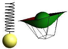
The following algorithm draws a spiral with a cone that point towards an increasing t on the spiral, in "pseudo code":

   // draw the helix with 10 windings
   double b=0.5;
   double ht=0.0;
   glBegin(GL_LINE_STRIP);
   while(ht<10.0)
   {
      glVertex3d(cos(ht*2*PI),sin(ht*2*PI),b*ht);
      ht+=0.02;
   }
   glEnd();

   // set up the 4 vectors we need for the Frenet Frame at t
   double n=sqrt(1+b*b);
   // the normalized derivative, tangent
   double T[]={-sin(t)/n,cos(t)/n,b/n,0.0};
   // the normalized cross product T x the double derivative
   double B[]={b*sin(t)/n,-b*cos(t)/n,1/n,0.0};
   // TxB, normalized
   double N[]={-cos(t),-sin(t),0.0,0.0};
   // and the origo
   double C[]={cos(t),sin(t),b*t,1.0};


   // set the matrix, NOTE: transposed compared to theory above
   double M[]={
               N[0],N[1],N[2],N[3],
               T[0],T[1],T[2],T[3],
               B[0],B[1],B[2],B[3],
               C[0],C[1],C[2],C[3],
              };

   // draw the cylinder at position C[t]
   glPushMatrix();
   glMultMatrixd(M);
   qdh=gluNewQuadric();
   gluCylinder(qdh,0.0f,0.2f,0.3f,15,15);
   gluDeleteQuadric(qdh);
   glPopMatrix();

A Bezier curve example

We'll have a closer look at a more general curve shape: The Bezier curve. We will study a cubic curve. We know that the Bezier curve, the derived and the double derived can be represented like this (we use C to indicate the curve to use the same term as above):

C(t)= P0(-t³+3t²-3t+1) + P1(3t³-6t²+3t) + P2(-3t³+3t²) + P3(t³)
C'(t)= P0(-3t²+6t-3) + P1(9t²-12t+3) + P2(-9t²+6t) + P3(3t²)
C''(t)=P0(-6t+6) + P1(18t-12) + P2(-18t+6) + P3(6t)

Methodical

We will not calculate analytically all the vectors we need. This can just as well be done numerically, in the application. We use the same method as we did with the spiral:

   			T=C'
   			B=T x C''
  		 	N=T x B
   		

If we carry out the reasoning as before we will get a problem with the orientation of the axes. If we draw the axes as we find them we will get a result like the one to the right. This is due to the use of the double derived as a foundation for calculating B. The double derived changes direction on the way. The consequence of this is not noticeable if the figure we draw is the same in the zx and zy projection.

We can search for a correction of this by finding another vector than the double derived when we decide B. For example we can try using V=(0.0 , 0.0 , 1.0 , 0.0).

   			T=C'
   			B=T x V
   			N=T x B
	   

Whether these are the directions we want is a different issue, but at least we have avoided the sudden, uncontrolled change in the axes' directions. A closer analysis of the anatomy in these Frenet matrices can help us to find desired solutions. For one thing we can instead of writing M=|B N T C| write M=|T B N C| and as a result we can put the x-axis along the tangent.

Algorithm

The application tube tube.zip puts short cylinders along a Bezier curve. A reasonably nice-looking tube is dependant on the length of the cylinder and the lengths between them.

Because of our choice to calculate the vectors numerically we need an apparatus to calculate cross products of vectors and to normalize vectors. If we in addition are going to draw the Bezier function by hand, we need some help methods to calculate Bezier values. The algorithm below is a coarse sketch based on CStdView::DrawScene in the application called tube.

// Bezier, Derivative of Bezier and
// double derivative are all prepared in
// bez, d_bez and dd_bez

// the Bezier function
CMaterial::SetMaterial(RED_PLASTIC);
glLineWidth(4);
drawBezier();

// do the t-walk and draw in frenet frames
int ix=0;
while(ix<PCNT)
{

   // Bezier is now tabulated in:
   // (bez[ix][0],bez[ix][1],bez[ix][2])
   // The derivative (tangent) is tabulated in:
   // (d_bez[ix][0],d_bez[ix][1],d_bez[ix][2])
   // The double derivate is tabulated in:
   // (dd_bez[ix][0],dd_bez[ix][1],dd_bez[ix][2])

   // finding the normalized tangent:
   // T pointing along the curve
   v3d T(d_bez[ix][0],d_bez[ix][1],d_bez[ix][2]);
   T.normalize();

   // finding the normalized d cross dd vector:
   // B pointing perpendicular to T
   v3d B(d_bez[ix][0],d_bez[ix][1],d_bez[ix][2]);
   B.cross(dd_bez[ix][0],dd_bez[ix][1],dd_bez[ix][2]);
   B.normalize();

   // if we are not happy with the double derivative
   // as basis for the second vector
   // maybe we can use an other vector here?
   // what is the effect of a fixed direction?
   // B.cross(0.0f,0.0f,1.0f);
   // B.normalize();

   // finding a third perpendiculat vector:
   // N perpendicular to both T and B
   v3d N(B.x,B.y,B.z);
   N.cross(T);  // and it is normalized since B and T are

   // we want to move to the correct point on the Bezier curve
   // as tabulated in (bez[ix][0],bez[ix][1],bez[ix][2])
   v3d C(bez[ix][0],bez[ix][1],bez[ix][2]);

   // at this point T,B,N describes the coordinate system
   // we will use at the position C
   // N will act as x-axes
   // B will act as y-axes
   // T will act as z-axes

   // setting up the matrix that will take us to the
   // Frenet frame located at this t-point
   // M=|N,B,T,C|, where C is the Bezier itself
   // note transpose of matrix

   GLfloat M[16]={
      N.x,N.y,N.z,0,
      B.x,B.y,B.z,0,
      T.x,T.y,T.z,0,
      C.x,C.y,C.z,1
   };

   glPushMatrix();
   glMultMatrixf(& M[0]);
   // and we are ready to draw what ever we want to draw
   // the green tubes
   // draw a cylinder as a temporary solution
   GLUquadricObj *glpQ=gluNewQuadric();
   CMaterial::SetMaterial(EMERALD);
   gluCylinder(glpQ,1.1f,1.1f,1.0f,15,1);
   gluDeleteQuadric(glpQ);
   glPopMatrix();

   ix++;
}
 		

General

In both examples we have looked at functions that are analytical described and possible to derive. We have used this when we have calculated on of the axes as the curves tangent. The spiral is a special example. The Bezier curve gives us much flexibility and is useful in general. We can imagine other functions with the same nice qualities. Examples are curves described with trigonometric functions.

We can in the meantime imagine an equivalent problem in a situation where the curve is described by a series of points. In this case we have no analytical way to find the derived. We can use the same reasoning in these cases. The problem with finding the tangent is a little different. If there is a relation between the lists of points, meaning that they describe some sort of trajectory, we may be able to use the vector from one point to the next as a tangent. If this is not the case we have another and completely open situation and the criteria for choosing the directions for the axes would be different and depending upon the situation.

An interesting case where we can consider the use of Frenet Frames is when we want figure B in position PB to be oriented towards figure A in position PA when figure A moves. The vector PB->PA would in this case serve as a candidate for one of the axes in the Frenet coordinate system, which is the coordinate system we want to draw B in.